exponential curve fitting

Exponential Curve Fitting

	download exerciser program
	download complete Delphi-7 project
	see source code of curve fitting

Introduction

This new article describes the exponential curve fitting method implemented in Graphics-Explorer,
my equations grapher program.
It replaces the old article, which can be found [here].
New is an exerciser program allowing step by step observation of the curve fitting process.

The curve fitter calculates the best fitting exponential function given a set of points.
This function is

y = a.b^x + c

where a,b,c are called the parameters.

Contents

exerciser description

curve fitting theory

project description

Exerciser description

Below is a reduced picture of the exerciser at work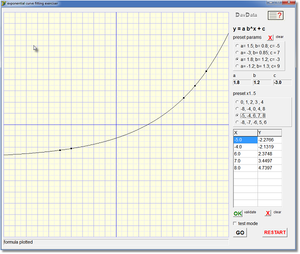

a,b,c		calculated parameters. (black:valid; red:invalid)
preset params		click radio button to preset parameters
preset x1..x5		click radio button to preset points
x, y		list of points, maximum is 10
[OK] validate		click to check/organize points prior to calculation
[GO]		start calculation of parameters a,b,c
[ ] testmode		mark to watch step by step calculation

Operation

Points can be added by:

After changing points in any way, click the [OK] button to check and to sort the points.
To watch the process step by step, mark the [testmode] checkbox.
Then click the [GO] button to calculate the a,b,c parameters and paint the graph.
To clear parameters or points, click the appropriate [X] button or [RESTART].

Curve fitting theory

Input to the curve fitter is a set of points [x₁,y₁]....[x_n,y_n]
The minimal required number of points is 3.
The maximum number of points is 10.
The fitter calculates parameters a,b,c such that the curve y = a.b^x + c has the smallest distance to these points.

For internal computations y = a.e^bx + c is used (e^b is reported for b)
The method has a numerical and an analytical part.
These are the steps:

^bx

least square

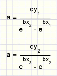
approximation of b

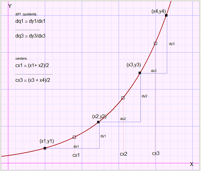
array dx holds the x differences between adjacent points
dx1 = x2 - x1....dx3 = x4 - x3

array dy holds the y differences
dy1 = y2 - y1....dy3 = y4 - y3

array cx holds the centers between points
cx1 = (x1+x2)/2....cx3 = (x3+x4)/2

array dq holds the differential quotients
dq1 = dy1/dx1....dq3 = dy3/dx3

Note: in the Delphi language, cx1 is written as cx[1]...etc.

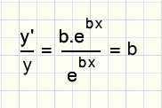
Starting with

^bx

which eliminates c.
So, we may write

₁

^bx₁

₂

^bx₂

₃

^bx₃

Parameter a can be eliminated by division of subsequent y':

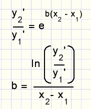
with above arrays in mind:

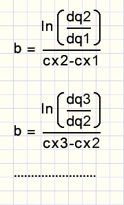
The center values (cx) are used, because the tangent (differential quotient dq) is most accurate
between two x values.
For subsequent points, the average value of b is calculated.
This is the approximation of b.

approximation of a

Starting with

₁

^bx₁

₂

^bx₂

we may eliminate c by subtraction of subsequent rows:

₂

₁

^bx₂

^bx₁

so....

An average value of a is calculated.
This is the approximation of a.

approximation of c

^bx

We may write

₁

^bx₁

₂

^bx₂

An avarage value of c is calculated.
This is the approximation of c.

Intermezzo

In equation

the value of y will increase by a factor g if x increases by 1.
g is called the growth factor.

Exponential functions (having c=0, the x-axis is the horizontal asymptote), are the result
of constant relative growth.

In equation

^bx

we notice that g = e^b.
b is called the relative growth speed because

So, if a function has a constant relative growth speed of b, it's growth factor g = e^b
where e is the base of the natural logarithm. (e = 2.71828....)

Before, we have obtained an approximation of c so we may write ...y - c = ae^bx
If the points (x1,y1)...(xn,yn) are on a true exponential function,
we will find the same growth factor, comparing subsequent points.
In the next part, fine tuning of c, we are going to vary c to obtain the smallest
deviation in growth factors.

fine tuning c

At this point we forget the a and b values and continue with c and the points [x1,y1]...[xn,yn].

For a certain value of c we write

₁

^bx₁

₂

^bx₂

division eliminates a

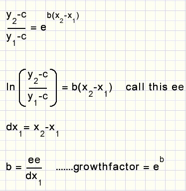
Two successive points produce a value of ee.
The values of ee are summed in variable AVG, for now AVG = ee1 + ee2 + ....
The growthfactors are stored in array growthfactor:
growthfactor1 = e^ee/dx1..........

By summing the ee values, we actually sum values b.dx1 + b.dx2 + b.dx3... = b(last X - first X)
So, b = AVG / (last X - first X)
Average growth factor is e^b

^{AVG/(lastX-firstX)}

Next, we have to compare the values in the growthfactor array with AVG.
Deviation = abs(AVG-growthFactor1) + abs(AVG-growthfactor2) + ......
Deviation is the result of procedure deviation which is called for a certain value of c.

least square method

The least-square-method is an algorithm to calculate the best fitting polynomial y = c₀ + c₁x + c₂x²+ ....
given a set of points.
With a final value of c, we may write

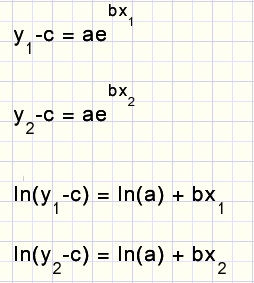
which represents a linear function like y = a + bx.
We present the points (ln(y_i-c),x_i) to the least square procedures to obtain the best a,b values.
Resulting a is replaced by e^a to cancel the ln( ) function.

The least square method is a nice application of linear algebra.
Look [here] for a description.

Aborts

The deviation procedure produces an abort if c is between two y values.
In that case y = c intersects the curve.
c must be outside the range y1, y2,y3.....

A negative or zero ee value does not allow for an ln function.
Below is the flowchart for the fine tuning of c

DeltaC is the increment value of c.
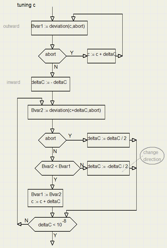
The fine tuning ends when deltaC has become very small.

Watchdog timer

Procedure morepointsexp controls the calculation of the a,b,c parameters.
Floating point operation are between try...except directives.
There are 2 cases for an abort:
1.Illegal Floating point operation
This situation occurs if the points are too far off to make an exponential function
an example being (1,1) , (5,5) , (8,2)

2.C runaway
If C is too far out, an even further position may yield a smaller growth factor deviation.
So, C "runs away".
The watchdog counter w ends this process.
Fine tuning of c must be completed in maximal 100 steps, otherwise the process is aborted.
This situation occurs in case of sharp bends.

The Delphi-7 project

There are 4 units and 1 form:

Unit1

Graphs are painted in bitmap map, points are painted on paintbox1.
The dimension is 800*800 pixels, coordinate (0,0) is at map position (400,400).
x domain is -10< x < 10,.........y range is -10< y <10.
The scale is 40:1.
There are 2 important flags:

If paramsOK = true, pressing [GO] just plots the function.
If paramsOK = false, pressing [GO] calculates a,b,c and then plots the function.
if parameters a,b,c do not represent the actual situation, they are painted in red.

Please refer to the source code for details.

Unit2

Main call is made to procedure makeExpFunction.
Points are collected from unit1 and stored in array Epoints[ ] of type Tpnt.

type TPnt = record
             x,y : double;
            end;

procedure deviation calculates the variation of growthfactors while fine tuning c.
These values are stored in variables Bvar1,Bvar2.

Unit3

Unit2 calls procecures in unit3 to display the steps in the curve fitting process.
Information is written in form1 paintbox1.
The waitflag : boolean (in unit1) controls the step-by-step action.
While the waitflag is true, the program executes the processmessages procedure.

Unit4

Has the necessary procedures for the least square method.
Main call is to procedure buildexp12(var pp : Tpoints; maxp : byte),
where Tpoints is the array of points and maxp the number of points supplied.

This concludes the description.